4 Reproduce Work

4.1 Minimize Error

We have already seen how the right set of tools can save you time by automatically highlighting the syntax of your code, ensuring everything you cite ends up in your bibliography, picking out mistakes in syntax, and providing templates for commonly-used methods or functions. Your time is saved twice over: you don’t repeat yourself, and you make fewer errors you’d otherwise have to fix. When it comes to managing ongoing projects, minimizing error means addressing two related problems. The first is to find ways to further reduce the opportunity for errors to creep in without you noticing. This is especially important when it comes to coding and analyzing data. The second is to find a way to figure out, retrospectively, what it was you did to generate a particular result. Using a revision control system gets us a good distance down this road. But there is more we can do at the level of particular reports or papers.

When you write code it is often in the process of doing some analysis on the fly. Ideas occur to you, you have a few things you want to look at, one thing leads to another. As a rule, you should try to document your work as you go. If you are writing an R script, then this usually means adding (brief, but useful) comments to your work to explain what it is a piece of code is meant to do. Is should also mean trying to write your code so that is readable. Code is like prose in this respect. Hadley Wickham’s R Style Guide provides some useful guidelines about writing readable code. The R package lintr implements these principles—it acts like a copy-editor for your code. In Emacs you can use lintr automatically through a tool called flycheck.

You should also try not to repeat yourself when you write your code. A good rule is that if you find yourself copying and pasting chunks of code (for example, to draw the same sort of plot or run the same kind of model for a bunch of different variables) then you should pause and see if you can write a quick convenience function instead to automate things more effectively. That way, your code can be shorter and also less prone to the errors and inconsistencies that creep in through repeated copy-and-paste.

4.2 From Server Farm to Data Table

Errors in data analysis often well up out of the gap that typically exists between the procedure used to produce a figure or table in a paper and the subsequent use of that output later. In the ordinary way of doing things, you have the code for your data analysis in one file, the output it produced in another, and the text of your paper in a third file. You do the analysis, collect the output and copy the relevant results into your paper, often manually reformatting them on the way. Each of these transitions introduces the opportunity for error. In particular, it is easy for a table of results to get detached from the sequence of steps that produced it. Almost everyone who has written a quantitative paper has been confronted with the problem of reading an old draft containing results or figures that need to be revisited or reproduced (as a result of peer-review, say) but which lack any information about the circumstances of their creation. Academic papers take a long time to get through the cycle of writing, review, revision, and publication, even when you’re working hard the whole time. It is not uncommon to have to return to something you did two years previously in order to answer some question or other from a reviewer. You do not want to have to do everything over from scratch in order to get the right answer. I am not exaggerating when I say that, whatever the challenges of replicating the results of someone else’s quantitative analysis, after a fairly short period of time authors themselves find it hard to replicate their own work. Computer Science people have a term of art for the inevitable process of decay that overtakes a project simply in virtue of its being left alone on the hard drive for six months or more: bit–rot.

4.3 Use RMarkdown and knitr

An important way to caulk this gap is to use RMarkdown and knitr when doing quantitative analysis in R. We’ve already seen how to write plain-text documents in Markdown’s lightweight format. RMarkdown allows you to incorporate code into this process. It is designed to integrate the plain-text documentation or writeup of a data analysis and its execution. You write the text of your paper (or, more often, your report documenting a data analysis) as normal. Whenever you want to run a model, produce a table or display a figure, rather than paste in the results of your work from elsewhere, you write down the R code that will produce the output you want. These “chunks” of code can be interspersed throughout the document. They are distinguished from the regular text by a special delimiter at the beginning and end of the block.

When you’re ready, you knit the document (Xie, 2015). That is, you feed your .Rmd file to R, which processes the code chunks, and produces a new .md where the code chunks have been replaced by their output. You can then turn that Markdown file into a PDF or HTML document. Relatedly, the rmarkdown library in R provides a render() function that takes you from .Rmd to HTML or PDF in a single step. This is what RStudio uses to produce your documents. Conversely, if you just want to extract the code you’ve written from the surrounding text, then you “tangle” the file, which results in an .R file. It’s pretty straightforward in practice. The strength of this approach is that is makes it much easier to document your work properly. There is just one file for both the data analysis and the writeup. The output of the analysis is created on the fly, and the code to do it is embedded in the paper. If you need to do multiple but identical (or very similar) analyses of different bits of data, RMarkdown and knitr can make generating consistent and reliable reports much easier.

RMarkdown is one of several “literate programming” formats. The idea goes back to Donald Knuth, the pioneering theorist of computer science who developed the TeX typesetting system in his spare time. Although his focus was on documenting computer programs, in retrospect Knuth anticipated many of the main ideas—and developed several of the initial tools—for reproducible data analysis.

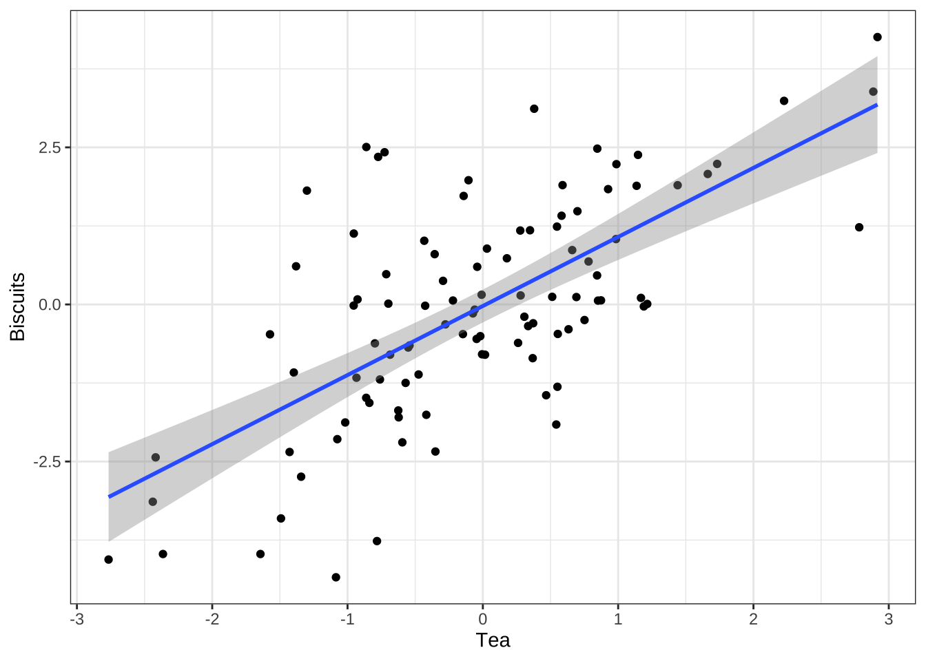
Figure 4.1, for instance, could be generated on the fly from source-code blocks included in the .Rmd source for this article. Sometimes we will want to only show the results produced by the code—in this case, Figure 4.1. But at other times we will want to display the code as well, as here.

library(ggplot2)
tea <- rnorm(100)
biscuits <- tea + rnorm(100, 0, 1.3)
data <- data.frame(tea, biscuits)
p <- ggplot(data, aes(x = tea, y = biscuits)) +
    geom_point() + 
    geom_smooth(method = "lm") + 
    labs(x = "Tea", y = "Biscuits") + theme_bw() 
print(p)

The knitr library and RMarkdown make it easy to produce HTML output, too. This makes for easy portability, conversion, and quick previewing while editing. You can work with RMarkdown files in any text editor, and Emacs has strong support for them. RStudio also comes with built-in support for .Rmd files and makes it very easy to produce HTML and PDF output, and to publish your reports to the web via its RPubs service.⁷

The knitr website has numerous examples showing how it works. These range from the basic setup to more developed examples.

The literate programming approach has its limits. For large or complex analyses it can still make more sense to produce the final result in pieces rather than all at once in a single .Rmd file. This is one of the reasons it remains important to manage your projects using some kind of version control, so you can keep track of work that is needed but might not fit inside a single .Rmd document.